By Amanda Rigdon

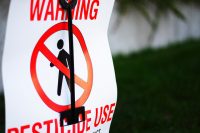
Almost as soon as cannabis became recreationally legal, the public started to ask questions about the safety of products being offered by dispensaries – especially in terms of pesticide contamination. As we can see from the multiple recalls of product there is a big problem with pesticides in cannabis that could pose a danger to consumers. While The Nerd Perspective is grounded firmly in science and fact, the purpose of this column is to share my insights into the cannabis industry based on my years of experience with multiple regulated industries with the goal of helping the cannabis industry mature using lessons learned from other established markets. In this article, we’ll take a look at some unique challenges facing cannabis testing labs, what they’re doing to respond to the challenges, and how that can affect the cannabis industry as a whole.

The Big Challenge

Over the past several years, laboratories have quickly ‘grown up’ in terms of technology and expertise, improving their methods for pesticide detection to improve data quality and lower detection limits, which ultimately ensures a safer product by improving identification of contaminated product. But even though cannabis laboratories are maturing, they’re maturing in an environment far different than labs from regulated industry, like food laboratories. Food safety testing laboratories have been governmentally regulated and funded from almost the very beginning, allowing them some financial breathing room to set up their operation, and ensuring they won’t be penalized for failing samples. In contrast, testing fees for cannabis labs are paid for by growers and producers – many of whom are just starting their own business and short of cash. This creates fierce competition between cannabis laboratories in terms of testing cost and turnaround time. One similarity that the cannabis industry shares with the food industry is consumer and regulatory demand for safe product. This demand requires laboratories to invest in instrumentation and personnel to ensure generation of quality data. In short, the two major demands placed on cannabis laboratories are low cost and scientific excellence. As a chemist with years of experience, scientific excellence isn’t cheap, thus cannabis laboratories are stuck between a rock and a hard place and are feeling the squeeze.

Responding to the Challenge

One way for high-quality laboratories to win business is to tout their investment in technology and the sophistication of their methods; they’re selling their science, a practice I stand behind completely. However, due to the fierce competition between labs, some laboratories have oversold their science by using terms like ‘lethal’ or ‘toxic’ juxtaposed with vague statements regarding the discovery of pesticides in cannabis using the highly technical methods that they offer. This juxtaposition can then be reinforced by overstating the importance of ultra-low detection levels outside of any regulatory context. For example, a claim stating that detecting pesticides at the parts per trillion level (ppt) will better ensure consumer safety than methods run by other labs that only detect pesticides at concentrations at parts per billion (ppb) concentrations is a potentially dangerous claim in that it could cause future problems for the cannabis industry as a whole. In short, while accurately identifying contaminated samples versus clean samples is indeed a good thing, sometimes less isn’t more, bringing us to the second half of the title of this article.

Less isn’t always more…

In my last article, I illustrated the concept of the trace concentrations laboratories detect, finishing up with putting the concept of ppb into perspective. I wasn’t even going to try to illustrate parts per trillion. Parts per trillion is one thousand times less concentrated than parts per billion. To put ppt into perspective, we can’t work with water like I did in my previous article; we have to channel Neil deGrasse Tyson.

The Milky Way galaxy contains about 100 billion stars, and our sun is one of them. Our lonely sun, in the vastness of our galaxy, where light itself takes 100,000 years to traverse, represents a concentration of 10 ppt. On the surface, detecting galactically-low levels of contaminants sounds wonderful. Pesticides are indeed lethal chemicals, and their byproducts are often lethal or carcinogenic as well. From the consumer perspective, we want everything we put in our bodies free of harmful chemicals. Looking at consumer products from The Nerd Perspective, however, the previous sentence changes quite a bit. To be clear, nobody – nerds included – wants food or medicine that will poison them. But let’s explore the gap between ‘poison’ and ‘reality’, and why that gap matters.

In reality, according to a study conducted by the FDA in 2011, roughly 37.5% of the food we consume every day – including meat, fish, and grains – is contaminated with pesticides. Is that a good thing? No, of course it isn’t. It’s not ideal to put anything into our bodies that has been contaminated with the byproducts of human habitation. However, the FDA, EPA, and other governmental agencies have worked for decades on toxicological, ecological, and environmental studies devoted to determining what levels of these toxic chemicals actually have the potential to cause harm to humans. Rather than discuss whether or not any level is acceptable, let’s take it on principle that we won’t drop over dead from a lethal dose of pesticides after eating a salad and instead take a look at the levels the FDA deem ‘acceptable’ for food products. In their 2011 study, the FDA states that “Tolerance levels generally range from 0.1 to 50 parts per million (ppm). Residues present at 0.01 ppm and above are usually measurable; however, for individual pesticides, this limit may range from 0.005 to 1 ppm.” Putting those terms into parts per trillion means that most tolerable levels range from 100,000 to 50,000,000 ppt and the lower limit of ‘usually measurable’ is 10,000 ppt. For the food we eat and feed to our children, levels in parts per trillion are not even discussed because they’re not relevant.

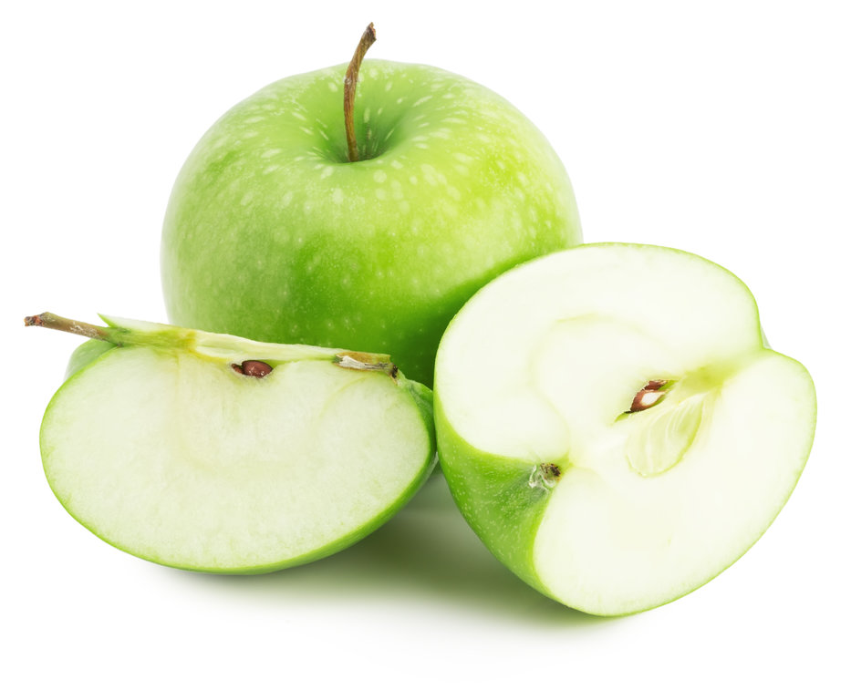
A specific example of this is arsenic. Everyone knows arsenic is very toxic. However, trace levels of arsenic naturally occur in the environment, and until 2004, arsenic was widely used to protect pressure-treated wood from termite damage. Because of the use of arsenic on wood and other arsenic containing pesticides, much of our soil and water now contains some arsenic, which ends up in apples and other produce. These apples get turned into juice, which is freely given to toddlers everywhere. Why, then, has there not an infant mortality catastrophe? Because even though the arsenic was there (and still is), it wasn’t present at levels that were harmful. In 2013, the FDA published draft guidance stating that the permissible level of arsenic in apple juice was 10 parts per billion (ppb) – 10,000 parts per trillion. None of us would think twice about offering apple juice to our child, and we don’t have to…because the dose makes the poison.

How Does This Relate to the Cannabis Industry?

The concept of permissible exposure levels (a.k.a. maximum residue limits) is an important concept that’s understood by laboratories, but is not always considered by the public and the regulators tasked with ensuring cannabis consumer safety. As scientists, it is our job not to misrepresent the impact of our methods or the danger of cannabis contaminants. We cannot understate the danger of these toxins, nor should we overstate their danger. In overstating the danger of these toxins, we indirectly pressure regulators to establish ridiculously low limits for contaminants. Lower limits always require the use of newer testing technologies, higher levels of technical expertise, and more complicated methods. All of this translates to increased testing costs – costs that are then passed on to growers, producers, and consumers. I don’t envy the regulators in the cannabis industry. Like the labs in the cannabis industry, they’re also stuck between a rock and a hard place: stuck between consumers demanding a safe product and producers demanding low-cost testing. As scientists, let’s help them out by focusing our discussion on the real consumer safety issues that are present in this market.

*average of domestic food (39.5% contaminated) and imported food (35.5% contaminated)

October 6, 2016

The Nerd Perspective

Detecting the Undetectable

By Amanda Rigdon

4 Comments

In my last column, I took a refreshing step out of the weeds of the specifics behind cannabis analyses and took a broader, less technical look at the cannabis industry. I had envisioned The Nerd Perspective being filled with profound insights that I have had in the cannabis industry, but I have realized that if I restricted this column to insights most would consider profound…well…there would not be many articles. So in this article, I want to share an insight with you, but not one that is earth shattering. Instead, I want to talk about a simple concept in a way that might help you think a little differently about the results your lab generates, the results you have to pay for or even the results printed on a cannabis product you might purchase.

This article is all about the simple concept of concentration – the expression of how much of something there is in relation to something else. We use expressions of concentration all the time – calories per serving, percent alcohol in beer, even poll results in the presidential election circus. Cannabis is not excluded from our flippant use of concentration terms – percent cannabinoid content, parts-per-million (ppm) residual solvents, and parts-per-billion (ppb) pesticides. Most of us know the definition of percent, ppm, and ppb, and we use these terms all the time when discussing cannabis analytical methods. During my career in analytical chemistry, it has occurred to me that parts per billion is a really infinitesimal amount…I know that intellectually, but I have never tried to actually visualize it. So being the nerd that I am, I went about comparing these often-used concentration terms visually in my kitchen.

I started by preparing a 1% solution of food coloring paste in water. This was accomplished by weighing out 5g of the food coloring and dissolving it into 500mL of water (about one teaspoon into a pint). The resulting solution was so dark it was almost black:

The picture above expresses the low end of what we care about in terms of cannabinoid concentration and a pretty normal value for a high-concentration terpene in cannabis.

I then took one teaspoon of that mixture and dissolved it into 1.32 gallons of water (5mL into 5000mL), resulting in a 10ppm solution of green food coloring in water:

I did not expect the resulting solution to be so light colored given the almost-black starting solution, but I did dilute the solution one thousand times. To put this into perspective, 10ppm is well above many state regulatory levels for benzene in a cannabis concentrate.

I then took one teaspoon of the almost-colorless 10ppm solution and dissolved that into another 1.32 gallons of water, resulting in a very boring-looking 10ppb solution of green food coloring in water:

Obviously, since I diluted the almost-colorless 10ppm solution a thousand times, the green food coloring cannot be seen in the picture above. As a reference, 10ppb is on the low end of some regulations for pesticides in food matrices, including – possibly – cannabis. I know the above picture is not really very compelling, so let’s think in terms of mass. The picture above shows eleven pounds of water. That eleven pounds of water contains 50 micrograms of food coloring…the weight of a single grain of sand.

To expand on the mass idea, let’s take a look at the total mass of cannabis sold legally in Colorado in 2015 – all 251,469 pounds of it. To express just how staggeringly small the figure of 10ppb is, if we assume that all of that cannabis was contaminated with 10ppb of abamectin, the total mass of abamectin in that huge amount of cannabis would be just 1.143g – less than half the mass of a penny.

To me, that is an extremely compelling picture. The fact is there are instruments available that can measure such infinitesimal concentrations. What’s more, these tiny concentrations can be measured in the presence of relatively massive amounts of other compounds – cannabinoids, terpenes, sugars, fats – that are always present in any given cannabis sample. The point I’d like to make is that the accurate measurement of trace amounts of cannabis contaminants including pesticides and residual solvents is an astounding feat that borders on magical. This feat is not magic though. It requires extremely delicate instrumentation, ultra-pure reagents, expert analysts, and labor-intensive sample preparation. It is far from trivial, and unlike magic, requires a large investment on the part of the laboratories performing this feat of science. Other industries have embraced this reality, and the cannabis industry is well on its way toward that end…hopefully this article will help put the job of the cannabis analytical lab into perspective.

September 6, 2016

The Nerd Perspective

‘Instant’ Cannabis Potency Testing: Different Approaches from Different Manufacturers

By Amanda Rigdon

5 Comments

This is the first piece of a regular column that CIJ has been so kind to allow me to write for their publication. Some readers might recognize my name from The Practical Chemist column in this publication. Since the inception of that column, I’ve finally taken the plunge into the cannabis industry as chief technical officer of Emerald Scientific. Unlike The Practical Chemist, I will not spend the entire first article introducing the column. The concept is simple: while I find the textbook-esque content of The Practical Chemist scintillating, I have a feeling that the content is a little too heavy to spring on someone who is looking for engaging articles over their precious coffee break. Instead, The Nerd Perspective will consist of less-technical writing focusing on my experience and insights for the cannabis industry as a whole. But don’t worry – I’m sure I will not be able to refrain from technical jargon altogether.

To kick off the column, I want to talk about instrumentation for ‘instant’ cannabis potency testing. At this point, it’s common knowledge in the cannabis analytics industry that the most accurate way to test cannabis potency is through extraction then analysis by HPLC-UV. I agree wholeheartedly with that sentiment, but HPLC analyses have one drawback: they can be either inexpensive or fast – not both. There are some instruments entering the market now that– while not as directly quantitative as HPLC-UV – promise to solve the inexpensive/fast conundrum. During my most recent trip to California, I was able to spend some quality time with two well-known instrument manufacturers: SRI Instruments and PerkinElmer, both of whom manufacture instruments that perform fast, inexpensive cannabis potency analyses. From my previous home at the heights of The Ivory Tower of Chromatography: Home of the Application Chemists, SRI and PE couldn’t be more different. But as seen through the eyes of a company who deals with a wide range of customers and analytical needs, it turns out that SRI and PE are much the same – not only in their open and honest support of the cannabis industry, but also in terms of their love of all things technical.

My first stop was SRI Instruments. They are a relatively small company located in an unassuming building in Torrance, CA. Only a few people work in that location, and I spent my time with Hugh Goldsmith (chief executive officer) and Greg Benedict (tech service guru). I have worked with these guys for a few years now, and since the beginning, I have lovingly referred to them as the MacGyvers of chromatography. Anyone familiar with SRI GCs knows that what they lack in aesthetics, they make up for in practicality – these instruments truly reflect Hugh and Greg’s character (that’s meant as a compliment).

SRI specializes in relatively inexpensive portable and semi-portable instruments that are easy to set up, easy to operate, and most importantly – engineered for a purpose. It’s actually really hard to manufacture an instrument that meets all three of these criteria, and the folks at SRI accomplish this with their passionate and unique approach to problem solving. What I love about these guys is that for them, nothing is impossible. Here’s an example: the price of the portable GC-FID instruments SRI builds is inflated because the instruments require separate – and pricey – hydrogen generators. That’s a big problem – hydrogen generators are all pretty much the same, and none of them are cheap. This didn’t faze SRI: they just decided to design their own super small on-board hydrogen generator capable of supplying hydrogen to a simple GC system for six hours with just 20mL of distilled water from the grocery store! I’m not kidding – I saw it in action on their new Model 420 GC (more on that in some future pieces). Was the final product pretty? Not in the least. Did it work? Absolutely. This kind of MacGyver-esque problem solving can only be done successfully with a deep understanding of the core principles behind the problem. What’s more, in order to engineer instruments like these, SRI has to have mastery over the core principles of not only chromatographic separation, but also of software development, electrical engineering, and mechanical engineering – just to name a few. These quirky, unassuming guys are smart. SRI is a company that’s been unapologetically true to themselves for decades; they’ll never be a contender for beauty queen, but they get the job done.

On the surface, PerkinElmer (PE) contrasts with SRI in almost every way possible. With revenue measured in billions of dollars and employees numbering in the thousands, PE is a behemoth that plays not only in the analytical chemistry industry but also in clinical diagnostics and other large industries. Where SRI instruments have a characteristic look of familiar homeliness, PE instruments are sleek and sexy. However, PerkinElmer and SRI are more alike than it would seem; just like the no-frills SRI, the hyper-technical PE instruments are engineered for a purpose by teams of very smart, passionate people.

With its modest price tag and manual sample introduction, the SRI Model 420 is engineered for lower throughput users to be a fast, simple, and inexpensive approach to semi-quantitative process control. The purpose of the instruments manufactured by PE is to produce the highest-quality quantitative results as quickly as possible for high-throughput labs. PE instruments are built using the best technology available in order to eke out every last ounce of quantitative accuracy and throughput possible. Fancy technology is rarely inexpensive, and neither is rigorous product development that can last years in some cases. In a way, PE is Doogie Howser to SRI’s MacGyver. Like MacGyver, Doogie is super smart, and his setting is a sterile hospital rather than a warzone.

I had a wonderful conversation with Tim Ruppel, PE’s headspace-GC specialist, on the sample introduction technology incorporated into the TurboMatrix Headspace Sampler, where I also learned that the basic technology for all PerkinElmer headspace-GC instruments was designed by the men who wrote The Book on headspace gas chromatography: Bruno Kolb and Leslie Ettre**. Later, I was able to get a much-needed lesson on FT-IR and the Spectrum Two IR Spectrometer from Brian Smith, PE’s spectroscopy expert, who actually wrote the book on quantitative spectroscopy***. Tim and Brian’s excitement over their technology mirrored that of Hugh and Greg. It turns out that SRI and PerkinElmer are more alike than I thought.

These two instrument manufacturers have addressed the fast/inexpensive conundrum of cannabis potency testing in two different ways: SRI’s instrument is extremely inexpensive, easy to operate, and will provide semi-quantitative values for THC, CBD, and CBN in just a few minutes; PE’s instrument is more expensive up front, but provides quantitative (though not directly quantitative) values for all of the major cannabinoids almost instantly, and requires almost no maintenance or consumables. These two instruments were designed for specific uses: one for inexpensive, easy use, and the other for more comprehensive results with a higher initial investment. The question consumers have to ask themselves is “Who do I need to solve my problem?” For some, the answer will be MacGyver, and for others, Doogie Howser will provide the solution – after all, both are heroes.

** B. Kolb, L. Ettre, Static Headspace-Gas Chromatography: Theory and Practice, John Wiley & Sons, Hoboken, NJ, 2006.

*** Brian C. Smith, Quantitative Spectroscopy: Theory and Practice, Elsevier, Boston, MA, 2002.

June 29, 2016

The Practical Chemist

Internal Standards– Turning Good Data Into Great Data

By Amanda Rigdon

2 Comments

Everyone likes to have a safety net, and scientists are no different. This month I will be discussing internal standards and how we can use them not only to improve the quality of our data, but also give us some ‘wiggle room’ when it comes to variation in sample preparation. Internal standards are widely used in every type of chromatographic analysis, so it is not surprising that their use also applies to common cannabis analyses. In my last article, I wrapped up our discussion of calibration and why it is absolutely necessary for generating valid data. If our calibration is not valid, then the label information that the cannabis consumer sees will not be valid either. These consumers are making decisions based on that data, and for the medical cannabis patient, valid data is absolutely critical. Internal standards work with calibration curves to further improve data quality, and luckily it is very easy to use them.

So what are internal standards? In a nutshell, they are non-analyte compounds used to compensate for method variations. An internal standard can be added either at the very beginning of our process to compensate for variations in sample prep and instrument variation, or at the very end to compensate only for instrument variation. Internal standards are also called ‘surrogates’, in some cases, however, for the purposes of this article, I will simply use the term ‘internal standard.’

Now that we know what internal standards are, lets look at how to use them. We use an internal standard by adding it to all samples, blanks, and calibrators at the same known concentration. By doing this, we now have a single reference concentration for all response values produced by our instrument. We can use this reference concentration to normalize variations in sample preparation and instrument response. This becomes very important for cannabis pesticide analyses that involve lots of sample prep and MS detectors. Figure 1 shows a calibration curve plotted as we saw in the last article (blue diamonds), as well as the response for an internal standard added to each calibrator at a level of 200ppm (green circles). Additionally, we have three sample results (red triangles) plotted against the calibration curve with their own internal standard responses (green Xs).

Figure 1: Calibration Curve with Internal Standard Responses and Three Sample Results

In this case, our calibration curve is beautiful and passes all of the criteria we discussed in the previous article. Lets assume that the results we calculate for our samples are valid – 41ppm, 303ppm, and 14ppm. Additionally, we can see that the responses for our internal standards make a flat line across the calibration range because they are present at the same concentration in each sample and calibrator. This illustrates what to expect when all of our calibrators and samples were prepared correctly and the instrument performed as expected. But lets assume we’re having one of those days where everything goes wrong, such as:

We unknowingly added only half the volume required for cleanup for one of the samples
The autosampler on the instrument was having problems and injected the incorrect amount for the other two samples

Figure 2 shows what our data would look like on our bad day.

Figure 2: Calibration Curve with Internal Standard Responses and Three Sample Results after Method Errors

We experienced no problems with our calibration curve (which is common when using solvent standard curves), therefore based on what we’ve learned so far, we would simply move on and calculate our sample results. The sample results this time are quite different: 26ppm, 120ppm, and 19ppm. What if these results are for a pesticide with a regulatory cutoff of 200ppm? When measured accurately, the concentration of sample 2 is 303ppm. In this example, we may have unknowingly passed a contaminated product on to consumers.

In the first two examples, we haven’t been using our internal standard – we’ve only been plotting its response. In order to use the internal standard, we need to change our calibration method. Instead of plotting the response of our analyte of interest versus its concentration, we plot our response ratio (analyte response/internal standard response) versus our concentration ratio (analyte concentration/internal standard concentration). Table 1 shows the analyte and internal standard response values for our calibrators and samples from Figure 2.

Table 1: Values for Calibration Curve and Samples Using Internal Standard

The values highlighted in green are what we will use to build our calibration curve, and the values in blue are what we will use to calculate our sample concentration. Figure 3 shows what the resulting calibration curve and sample points will look like using an internal standard.

Figure 3: Calibration Curve and Sample Results Calculated Using Internal Standard Correction

We can see that our axes have changed for our calibration curve, so the results that we calculate from the curve will be in terms of concentration ratio. We calculate these results the same way we did in the previous article, but instead of concentrations, we end up with concentration ratios. To calculate the sample concentration, simply multiply by the internal standard amount (200ppm). Figure 4 shows an example calculation for our lowest concentration sample.

Figure 4: Example Calculation for Sample Results for Internal-Standard Corrected Curve

Using the calculation shown in Figure 4, our sample results come out to be 41ppm, 302ppm, and 14ppm, which are accurate based on the example in Figure 1. Our internal standards have corrected the variation in our method because they are subjected to that same variation.

As always, there’s a lot more I can talk about on this topic, but I hope this was a good introduction to the use of internal standards. I’ve listed couple of resources below with some good information on the use of internal standards. If you have any questions on this topic, please feel free to contact me at amanda.rigdon@restek.com.

Resources:

When to use an internal standard: http://www.chromatographyonline.com/when-should-internal-standard-be-used-0

Choosing an internal standard: http://blog.restek.com/?p=17050

June 1, 2016

The Practical Chemist

Calibration Part II – Evaluating Your Curves

By Amanda Rigdon

No Comments

Despite the title, this article is not about weight loss – it is about generating valid analytical data for quantitative analyses. In the last installment of The Practical Chemist, I introduced instrument calibration and covered a few ways we can calibrate our instruments. Just because we have run several standards across a range of concentrations and plotted a curve using the resulting data, it does not mean our curve accurately represents our instrument’s response across that concentration range. In order to be able to claim that our calibration curve accurately represents our instrument response, we have to take a look at a couple of quality indicators for our curve data:

correlation coefficient (r) or coefficient of determination (r²)
back-calculated accuracy (reported as % error)

The r or r² values that accompany our calibration curve are measurements of how closely our curve matches the data we have generated. The closer the values are to 1.00, the more accurately our curve represents our detector response. Generally, r values ≥0.995 and r² values ≥ 0.990 are considered ‘good’. Figure 1 shows a few representative curves, their associated data, and r² values (concentration and response units are arbitrary).

Figure 1: Representative Curves and r2 values

Let’s take a closer look at these curves:

Curve A: This represents a case where the curve perfectly matches the instrument data, meaning our calculated unknown values will be accurate across the entire calibration range.

Curve B: The r² value is good and visually the curve matches most of the data points pretty well. However, if we look at our two highest calibration points, we can see that they do not match the trend for the rest of the data; the response values should be closer to 1250 and 2500. The fact that they are much lower than they should be could indicate that we are starting to overload our detector at higher calibration levels; we are putting more mass of analyte into the detector than it can reliably detect. This is a common problem when dealing with concentrated samples, so it can occur especially for potency analyses.

Curve C: We can see that although our r² value is still okay, we are not detecting analytes as we should at the low end of our curve. In fact, at our lowest calibration level, the instrument is not detecting anything at all (0 response at the lowest point). This is a common problem with residual solvent and pesticide analyses where detection levels for some compounds like benzene are very low.

Curve D: It is a perfect example of our curve not representing our instrument response at all. A curve like this indicates a possible problem with the instrument or sample preparation.

So even if our curve looks good, we could be generating inaccurate results for some samples. This brings us to another measure of curve fitness: back-calculated accuracy (expressed as % error). This is an easy way to determine how accurate your results will be without performing a single additional run.

Back-calculated accuracy simply plugs the area values we obtained from our calibrators back into the calibration curve to see how well our curve will calculate these values in relation to the known value. We can do this by reprocessing our calibrators as unknowns or by hand. As an example, let’s back-calculate the concentration of our 500 level calibrator from Curve B. The formula for that curve is: y = 3.543x + 52.805. If we plug 1800 in for y and solve for x, we end up with a calculated concentration of 493. To calculate the error of our calculated value versus the true value, we can use the equation: % Error = [(calculated value – true value)/true value] * 100. This gives us a % error of -1.4%. Acceptable % error values are usually ±15 – 20% depending on analysis type. Let’s see what the % error values are for the curves shown in Figure 1.

Table 1: % Error for Back-Calculated Values for Curves A – D

Our % error values have told us what our r² values could not. We knew Curve D was unacceptable, but now we can see that Curves B and C will yield inaccurate results for all but the highest levels of analyte – even though the results were skewed at opposite ends of the curves.

There are many more details regarding generating calibration curves and measuring their quality that I did not have room to mention here. Hopefully, these two articles have given you some tools to use in your lab to quickly and easily improve the quality of your data. If you would like to learn more about this topic or have any questions, please don’t hesitate to contact me at amanda.rigdon@restek.com.

May 3, 2016

The Practical Chemist

Calibration – The Foundation of Quality Data

By Amanda Rigdon

1 Comment

This column is devoted to helping cannabis analytical labs generate valid data right now with a relatively small amount of additional work. The topic for this article is instrument calibration – truly the foundation of all quality data. Calibration is the basis for all measurement, and it is absolutely necessary for quantitative cannabis analyses including potency, residual solvents, terpenes, and pesticides.

Just like a simple alarm clock, all analytical instruments – no matter how high-tech – will not function properly unless they are calibrated. When we set our alarm clock to 6AM, that alarm clock will sound reproducibly every 24 hours when it reads 6AM, but unless we set the correct current time on the clock based on some known reference, we can’t be sure when exactly the alarm will sound. Analytical instruments are the same. Unless we calibrate the instrument’s signal (the response) from the detector to a known amount of reference material, the instrument will not generate an accurate or valid result.

Without calibration, our result may be reproducible – just like in our alarm clock example – but the result will have no meaning unless the result is calibrated against a known reference. Every instrument that makes a quantitative measurement must be calibrated in order for that measurement to be valid. Luckily, the principle for calibration of chromatographic instruments is the same regardless of detector or technique (GC or LC).

Before we get into the details, I would like to introduce one key concept:

Every calibration curve for chromatographic analyses is expressed in terms of response and concentration. For every detector the relationship between analyte (e.g. a compound we’re analyzing) concentration and response is expressible mathematically – often a linear relationship.

Now that we’ve introduced the key concept behind calibration, let’s talk about the two most common and applicable calibration options.

Single Point Calibration

This is the simplest calibration option. Essentially, we run one known reference concentration (the calibrator) and calculate our sample concentrations based on this single point. Using this method, our curve is defined by two points: our single reference point, and zero. That gives us a nice, straight line defining the relationship between our instrument response and our analyte concentration all the way from zero to infinity. If only things were this easy. There are two fatal flaws of single point calibrations:

We assume a linear detector response across all possible concentrations
We assume at any concentration greater than zero, our response will be greater than zero

Assumption #1 is never true, and assumption #2 is rarely true. Generally, single point calibration curves are used to conduct pass/fail tests where there is a maximum limit for analytes (i.e. residual solvents or pesticide screening). Usually, quantitative values are not reported based on single point calibrations. Instead, reports are generated in relation to our calibrator, which is prepared at a known concentration relating to a regulatory limit, or the instrument’s LOD. Using this calibration method, we can accurately report that the sample contains less than or greater than the regulatory limit of an analyte, but we cannot report exactly how much of the analyte is present. So how can we extend the accuracy range of a calibration curve in order to report quantitative values? The answer to this question brings us to the other common type of calibration curve.

Multi-Point Calibration:

A multi-point calibration curve is the most common type used for quantitative analyses (e.g. analyses where we report a number). This type of curve contains several calibrators (at least 3) prepared over a range of concentrations. This gives us a calibration curve (sometimes a line) defined by several known references, which more accurately expresses the response/concentration relationship of our detector for that analyte. When preparing a multi-point calibration curve, we must be sure to bracket the expected concentration range of our analytes of interest, because once our sample response values move outside the calibration range, the results calculated from the curve are not generally considered quantitative.

The figure below illustrates both kinds of calibration curves, as well as their usable accuracy range:

This article provides an overview of the two most commonly used types of calibration curves, and discusses how they can be appropriately used to report data. There are two other important topics that were not covered in this article concerning calibration curves: 1) how can we tell whether or not our calibration curve is ‘good’ and 2) calibrations aren’t permanent – instruments must be periodically re-calibrated. In my next article, I’ll cover these two topics to round out our general discussion of calibration – the basis for all measurement. If you have any questions about this article or would like further details on the topic presented here, please feel free to contact me at amanda.rigdon@restek.com.

April 4, 2016

The Practical Chemist

Easy Ways to Generate Scientifically Sound Data

By Amanda Rigdon

1 Comment

I have been working with the chemical analysis side of the cannabis industry for about six years, and I have seen tremendous scientific growth on the part of cannabis labs over that time. Based on conversations with labs and the presentations and forums held at cannabis analytical conferences, I have seen the cannabis analytical industry move from asking, “how do we do this analysis?” to asking “how do we do this analysis right?” This change of focus represents a milestone in the cannabis industry; it means the industry is growing up. Growing up is not always easy, and that is being reflected now in a new focus on understanding and addressing key issues such as pesticides in cannabis products, and asking important questions about how regulation of cannabis labs will occur.

While sometimes painful, growth is always good. To support this evolution, we are now focusing on the contribution that laboratories make to the safety of the cannabis consumer through the generation of quality data. Much of this focus has been on ensuring scientifically sound data through regulation. But Restek is neither a regulatory nor an accrediting body. Restek is dedicated to helping analytical chemists in all industries and regulatory environments produce scientifically sound data through education, technical support and expert advice regarding instrumentation and supplies. I have the privilege of supporting the cannabis analytical testing industry with this goal in mind, which is why I decided to write a regular column detailing simple ways analytical laboratories can improve the quality of their chromatographic data right now, in ways that are easy to implement and are cost effective.

Anyone with an instrument can perform chromatographic analysis and generate data. Even though results are generated, these results may not be valid. At the cannabis industry’s current state, no burden of proof is placed on the analytical laboratory regarding the validity of its results, and there are few gatekeepers between those results and the consumer who is making decisions based on them. Even though some chromatographic instruments are super fancy and expensive, the fact is that every chromatographic instrument – regardless of whether it costs ten thousand or a million dollars – is designed to spit out a number. It is up to the chemist to ensure that number is valid.

In the first couple of paragraphs of this article, I used terms to describe ‘good’ data like ‘scientifically-sound’ or ‘quality’, but at the end of the day, the definition of ‘good’ data is valid data. If you take the literal meaning, valid data is justifiable, logically correct data. Many of the laboratories I have had the pleasure of working with over the years are genuinely dedicated to the production of valid results, but they also need to minimize costs in order to remain competitive. The good news is that laboratories can generate valid scientific results without breaking the bank.

In each of my future articles, I will focus on one aspect of valid data generation, such as calibration and internal standards, explore it in practical detail and go over how that aspect can be applied to common cannabis analyses. The techniques I will be writing about are applied in many other industries, both regulated and non-regulated, so regardless of where the regulations in your state end up, you can already have a head start on the analytical portion of compliance. That means you have more time to focus on the inevitable paperwork portion of regulatory compliance – lucky you! Stay tuned for my next column on instrument calibration, which is the foundation for producing quality data. I think it will be the start of a really good series and I am looking forward to writing it.